Some years ago I had the opportunity to participate in a Datawarehousing project with the SAP BW solution in a client of the food retail sector, the architecture they had was a BW 7.0 with Oracle database. As you can imagine, the volumetries were quite high, so we had to be very careful with the data model and apply the options that were available at that time to have an acceptable to good performance (compression, partitions, aggregates and performance-oriented queries).
One of the processes that had been defined was the creation of customer segments based on RFM segmentation which at that time was implemented with BW functionality and with static rules for the calculation of the segments; so in this post we are going to see an approach to perform RFM segmentation with a demo dataset but using native Hana functionality.
In this post with the first part I tell you about the physical and logical model and the approach with Hana AFM.
Part I: The model and RFM using Hana AFM
First of all, let’s start at the beginning.
What is RFM segmentation?
RFM segmentation is a very popular marketing technique that allows segmenting customers into groups with homogeneous behavior by analyzing purchase history in order to establish campaigns or actions adapted to the characteristics of each group.
Three axes of analysis are established:
- Recency (R): How recent is the customer’s visit or purchase (Date of last purchase).
- Frequency (F): Volume of purchase transactions (Number of transactions).
- Monetary (M): Amount of purchases (Amount).
The RFM can be used to answer questions such as:
- Who your best customers are.
- Customers likely to stop buying (churn).
- Which customers are in our interest to retain and which to let go (Pareto Principle applied to sales and marketing).
- ….
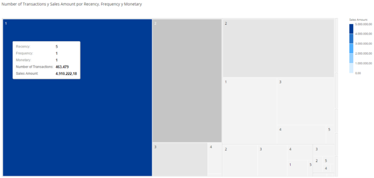
Let’s take a look at how RFM segmentation works. Given a dataset with sales history by customer. Given a dataset with sales history by customer.

We establish intervals by grouping the individual values, usually 5, to segment each of the 3 axes. The value 5 represents the segment with the most recent purchase (R), with the highest frequency (F) and with the highest monetary value (M) while the value 1 represents the segment with the oldest purchase (R), with the lowest frequency (F) and with the lowest monetary value (M).

Finally we determine the RFM segment by concatenating the value of each individual segment and calculate the score.
Score = (R + F + M) / 3

Let’s take a look at the elementsthat will be neededin our example.
- The physical data model: The tables with the loaded dataset.
- The logical data model: Model of views with calculations and relationships. The idea of this model is to service reporting and serve as a basis for the calculation of the RFM. The idea of this model is to service reporting and serve as a basis for the calculation of the RFM.
- Hana PAL for segment creation.
- Hana SDI (Smart Data Integration) for persistence.
- BI tool for visualization.
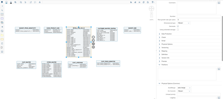
Physical data model
he data model we start from has a set of tables where one of them contains the transactional data of the sales tickets at item level with the sold product and others act as master data tables (attributes and descriptions). In our example we will work with a total of about 31 million transactional data records, 5.000 products and 50.000 customers.


Logical data model
To create the logical data model, we have opted for the functionality of Hana Modelling, creating a set of calculated views that has allowed us to create a virtual data model where we relate the tables, generate KPI’s and semantics on the fly at runtime.
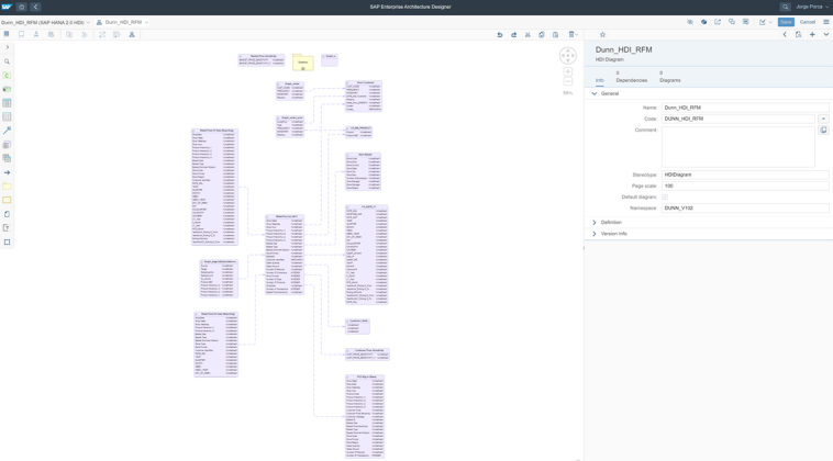
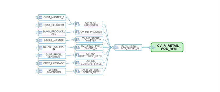
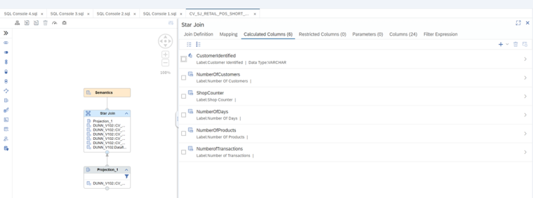
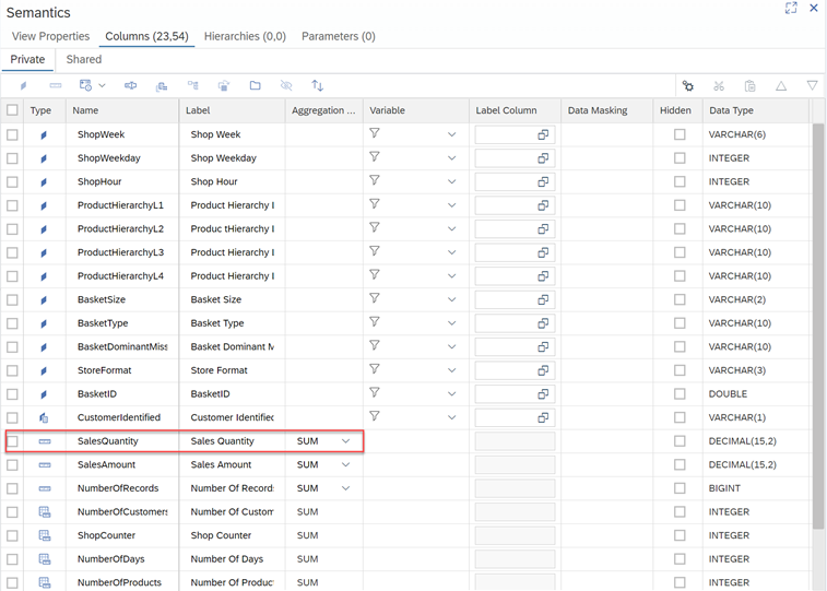
This set of views will provide us with the metrics we need to generate our RFM analysis as well as allowing us to exploit the information from BI tools, additionally we have a last view where we make the exposure of the fields that we will use in the segmentation (customer, amount, number of transactions and days since last purchase). The calculation detail of each one is as follows:
- For recency: We obtain it through a difference of dates between the time of analysis and the time of each of the purchases. As we are interested in the most recent purchase, we apply a ranking to keep the 1st purchase, i.e. the most recent one.

For the frequency: We obtain it by means of a ratio that applies a count distinct on the Ticket ID field, that is, we apply a count to know the number of tickets and therefore to know how many times the customer has made purchases in the selected time interval.

For the monetary: We obtain it through a decimal type ratio with sum aggregation method, it provides us with the amount of sales in the selected time interval.
Hana PAL (Binning) – Segments Creation
For the determination of segments it may be that we have been directly specified the number and how the intervals should be in each of them, in which case we will simply perform the definition in the implementation according to these rules.
For example create 5 intervals for the monetary segment with the following value ranges:
- From 0 – 100 — Segment 1.
- From 101 – 1000 — Segment 2.
- …
- From 100.000 a 200.000 — Segment 5.
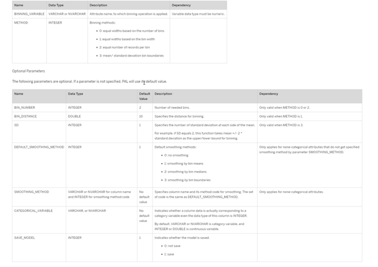
However, as part of the example in this post, what we are going to do instead of defining a series of manual intervals is to define them using the algorithms available in the Hana PAL, in particular we will use the Binning or discretization algorithm.
In this link (Hana Pal Binning) we have the detail of the options that can be applied to obtain intervals.
Binning Approach 1: AFM (Application Function Modeler)
The Application Function Modeler or AFM is a feature available in both Hana Studio (XS Classic) and Web IDE for Hana (XS Advance) that allows you to create a series of flows called flowgraphs that are implemented graphically to model and process data, selecting the source, the destination and a wide variety of operators in between. By default, the activation of a flowgraph generates a procedure in the system.
Some of the operators supported are the following:
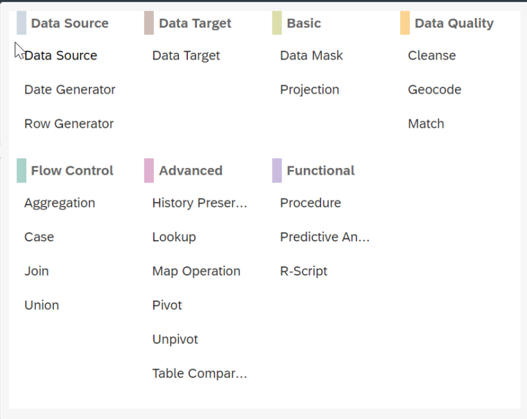

In our example we are going to implement 4 Flowgraphs to calculate the RFM, 3 of them will be used to obtain the R, the F and the M and the fourth one will be in charge of joining this information and persist it physically in a system table.
Recency
As a source we will select the key figure “Difference of days” that we have previously created in the view.

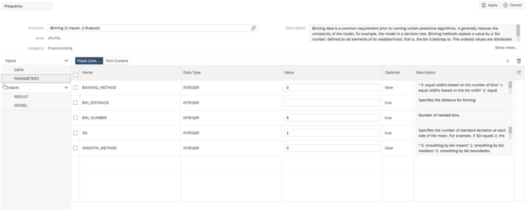
The binning configuration is as follows to generate 5 bins.

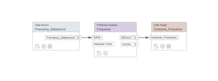
Frecuency
The binning configuration is as follows to generate 5 bins.

The binning configuration is as follows to generate 5 bins.
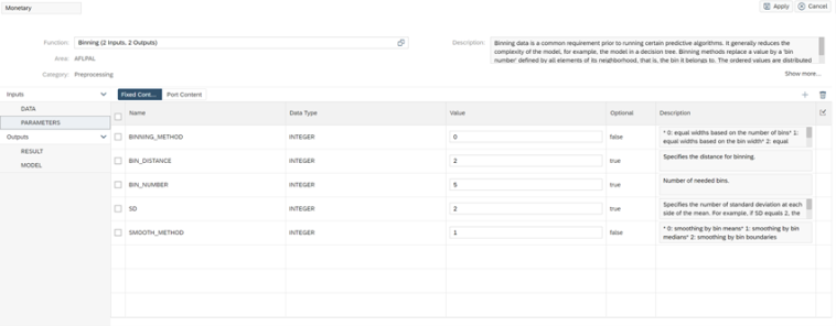
Monetary
As a source we select the key figure “Amount” that we have previously created in the view.
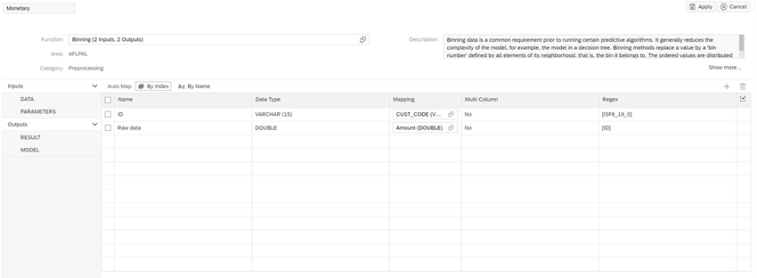
The binning configuration is as follows to generate 5 bins.
As a final step we have implemented a last flowgraph that will be in charge of joining the R, F and M previously calculated and persist them in a table in Hana.

Execute the process
The next step will be to execute our process this can be done in 2 ways either manually from each of the flowgraphs by pressing the “Execute” icon or through SQL script statements.

Once the process has been executed correctly, the appearance of the table where we will have all the clients perfectly categorized with each one of the intervals is the following.

At this point we have finished the example to perform a segmentation of RFM customers using the graphical functionality AFM (Application Function Modeler) through Flowgraphs.
In the next post I will tell you how to perform the same approach, but using the Python API for Machine learning algorithms in Hana and some interesting visualizations using a Live connection against this model from SAP Analytics Cloud (SAC) and thus being able to analyze the segments.